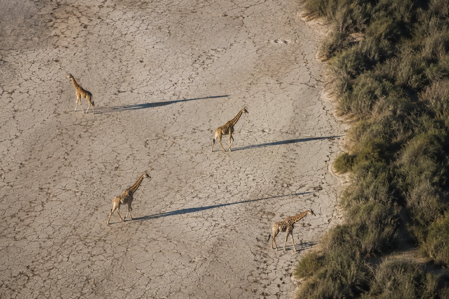
A giraffe is conspicuous beside a vehicle. From a moving aircraft, that same animal may be partly concealed by vegetation, briefly visible, or overlooked among other things an observer must record. The size of the animal does not tell us the size of the counting error. Nor does an aerial survey’s wide coverage guarantee that each part of the landscape is equally well represented.
Derek Lee and Monica Bond made that problem measurable in a 2016 study of Tanzania’s Tarangire ecosystem. They compared aerial estimates with two methods applied during the same ground surveys. Their work revealed more than a general shortfall from the air: disagreement varied enough among sites to change the apparent distribution of giraffe density.
That distinction matters to conservation. If a survey misses a larger fraction of animals in one place than another, it can make a valuable stronghold look ordinary. A correction needs to recover the geographical pattern as well as the overall number.
Two ways of reading the same ground encounters
Lee and Bond surveyed four areas with different land management: Tarangire National Park, Manyara Ranch Conservancy and two game-controlled areas. These were parts of a wider, mixed-use landscape rather than four identical enclosures. They compared their results with the most recent systematic reconnaissance flight, conducted in November 2011.
The ground team drove six repeated surveys between January and October 2012. The repetitions were organised as pairs near the end of each of three rainfall seasons. Returning over short intervals gave the team repeated opportunities to encounter the same animals, while spreading those visits through the year reduced dependence on the conditions of a single season.
At an encounter, they collected two different kinds of evidence. First, they measured the distance from the road to the giraffe or group. Animals become harder to see at greater distances, so the distribution of observed distances can help estimate how many were missed. This was the basis of their distance-sampling analysis.
Second, they photographed giraffes’ right sides. Individual coat patterns allowed photographs taken on different visits to be matched, producing a history of when each giraffe had been seen and missed. Capture–recapture analysis then used those histories to estimate both encounter probability and abundance. No physical mark had to be attached for this comparison.
The two analyses therefore began with overlapping field observations but asked different statistical questions. One inferred visibility from distance; the other inferred detection from individual reappearances. Agreement between them would be informative, and disagreement could expose problems hidden by using either one alone.
Keeping the biological units comparable
The ground comparison was restricted to adults because calves are particularly difficult to detect from aircraft. The field effort produced 503 distance records of adult groups and encounter histories for 1,347 recognizable adult giraffes. Those are different units: a group record can contain several animals, and an identified giraffe can appear on several surveys.
The aerial observers detected 82 giraffes in the comparison data. That raw tally was expanded through the aerial sampling design to estimate abundance over a much larger area. It should not be set directly beside 1,347 identified adults as though both numbers came from the same search effort. The useful comparison was between the estimates derived for corresponding areas.
There was another adjustment before that comparison. Earlier aerial surveys had produced lower giraffe estimates in the dry season than in the wet season. Lee and Bond applied a factor of 2.1 to put the 2011 dry-season estimate onto an estimated wet-season equivalent. The subsequent site-specific corrections addressed an additional gap between that season-adjusted aerial estimate and the photographic estimate.
The seasonal correction was not evidence that the giraffe population doubled when rain arrived. It adjusted a recurring difference in what the aerial survey measured. Keeping those stages separate prevents a methodological calculation from becoming a biological claim.
The missing animals were unevenly distributed
At three of the four sites, aerial estimates were significantly lower than estimates from photographic capture–recapture. The comparison was closest in Lolkisale Game Controlled Area and farthest apart in Mto wa Mbu Game Controlled Area. Rounded corrections to the season-adjusted aerial estimates ranged from 1.2 to 10.
| Site | Season-adjusted aerial adult-density estimate | Photographic adult-density estimate | Authors’ aerial correction factor |
|---|---|---|---|
| Tarangire National Park | 0.257 per km² | 0.777 per km² | 3.0 |
| Manyara Ranch comparison area | 0.235 per km² | 1.969 per km² | 8.4 |
| Lolkisale Game Controlled Area | 0.317 per km² | 0.363 per km² | 1.2 |
| Mto wa Mbu Game Controlled Area | 0.027 per km² | 0.272 per km² | 10.0 |
These estimates, reported in the paper’s Table 1, show the biological consequence particularly clearly at Manyara Ranch. The photographic analysis placed it well above the other sites in adult density. The aerial estimate did not reveal that contrast. The authors’ Figure 3 makes the same point visually: the height of the bars changes the apparent ranking of the landscape.
The ground methods did not agree everywhere either. Distance sampling gave a similar result to photographic analysis in Tarangire National Park, but the two differed significantly in Manyara Ranch and Lolkisale. Adding a detection model was an improvement, yet its particular assumptions still mattered. Vegetation, topography and clustering could affect observations in ways that distance alone did not capture.
Photographic estimates were the most precise of the three methods. Their average coefficient of variation, which expresses uncertainty relative to the size of the estimate, was 0.15, compared with 0.24 for distance sampling and 0.44 for aerial surveys. Narrower uncertainty can make a real future change easier to distinguish from ordinary survey variation.
A large correction still needs a boundary
When the researchers extended the corrections to the wider ecosystem, the earlier aerial estimate of 1,235 became approximately 7,844–7,902 giraffes under two alternative correction approaches. Those are the authors’ reconstructed estimates for the earlier survey period, not a population that grew sixfold between visits.
Crucially, Lee and Bond warned that the corrected total might exceed the true population. Their calibration sites could not represent every variation in habitat and density across the broader survey region, including places containing little usable giraffe habitat. Applying a correction established in giraffe habitat to a less suitable area could create animals on paper that were never there.
The study also lacked an independently known true population against which every estimator could be judged. The authors regarded photographic capture–recapture as their strongest reference because it modelled detection, recognized individuals and showed that the accumulation of new identities was levelling off. That is a reasoned choice of reference, not direct knowledge of every living giraffe.
Timing and access impose further limits. The ground surveys followed the flight by several months, so births, deaths or movements could contribute to differences. Road-based searches were also not randomly placed across the landscape. Animals’ attraction to, or avoidance of, roads could influence the ground result, particularly where people and livestock used those routes.
Together these constraints argue for local calibration and explicit habitat coverage. They do not erase the large discrepancies the researchers documented.
Recognizing individuals helps, but the model still matters
A later waterhole-camera comparison at Ongava in Namibia tested a different part of the same problem. Christophe Bonenfant, Ken Stratford and Stéphanie Périquet used one camera dataset to compare abundance models. They identified 101 giraffes, while their reference capture–recapture model estimated about 104. Other model choices produced estimates ranging from 87 to 215.
At Ongava, returning to drink was irregular: an animal photographed one day was less likely to be recorded the next. The observation process changed even though cameras stayed in fixed positions. That explains why photographs alone do not settle the counting problem; their analysis must reflect how the animals enter the sample.
The two studies provide complementary evidence. Tarangire compared aerial and ground observation systems across sites. Ongava held the main image collection constant and changed how those records were interpreted. Neither supplies a single correction that should be imposed everywhere. Both show why the method behind a giraffe estimate belongs beside its headline number.
Making a future trend interpretable
Lee and Bond proposed pairing broad aerial coverage with ground surveys that improve precision and calibrate detection. They also argued for methods that retain comparability with older records. A better survey can be a major improvement even when its first estimate cannot be read as a population trend.
One useful next comparison would repeat aerial and ground work close together across contrasting vegetation. That would help separate missed animals from changes occurring between survey dates. Another would ask whether corrections remain stable when the same area changes through drought, regrowth or altered land use. If visibility changes along with the habitat, an unchanged counting method can still produce a changing bias.
The practical achievement of the Tarangire study was to expose that bias with recognizable animals and repeated observations. Giraffe conservation needs to know where populations are most abundant and whether they are changing. Those answers become more credible when uncertainty in seeing an animal is measured rather than hidden inside the final total.
Sources
- Derek E. Lee and Monica L. Bond (2016). Precision, accuracy, and costs of survey methods for giraffe Giraffa camelopardalis. Journal of Mammalogy, 97, 940–948. DOI and journal record; full paper.
- Christophe Bonenfant, Ken Stratford and Stéphanie Périquet (2023). Counting giraffes: A comparison of abundance estimators on the Ongava Game Reserve, Namibia. Hystrix, the Italian Journal of Mammalogy, 34, 1–7. DOI; open manuscript.